Table Of Content
Such studies are extremely common, and there are several points worth making about them. First, non-manipulated independent variables are usually participant variables (private body consciousness, hypochondriasis, self-esteem, gender, and so on), and as such, they are by definition between-subjects factors. For example, people are either low in hypochondriasis or high in hypochondriasis; they cannot be tested in both of these conditions. Second, such studies are generally considered to be experiments as long as at least one independent variable is manipulated, regardless of how many non-manipulated independent variables are included. Third, it is important to remember that causal conclusions can only be drawn about the manipulated independent variable.
1.2. Measures of Different Constructs
Belong to the A × B interaction; interaction is absent (additivity is present) if these expressions equal 0.[13][14] Additivity may be viewed as a kind of parallelism between factors, as illustrated in the Analysis section below. As expected, we see that the average height is 1 inch taller when subjects wear shoes vs. do not wear shoes. So, the main effect of wearing shoes is to add 1 inch to a person’s height. All rights are reserved, including those for text and data mining, AI training, and similar technologies. For all open access content, the Creative Commons licensing terms apply. You have been employed by SuperGym, a local personal training gym, who want an engineer's perspective on how to offer the best plans to their clients.
2: Setting Up a Factorial Experiment
Optimization of Toluenediamine degradation in synthetic wastewater by a UV/H2O2 process using full factorial design - ScienceDirect.com
Optimization of Toluenediamine degradation in synthetic wastewater by a UV/H2O2 process using full factorial design.
Posted: Thu, 06 Jul 2023 07:35:04 GMT [source]
For wt% methanol in biodiesel, RPM is further from the blue line than pressure, which indicates that RPM has a more significant effect on wt% methanol in biodiesel than pressure does. After all the trials were performed, the wt% methanol remaining in the biodiesel and number of theoretical stages achieved were calculated. The figure below contains the DOE table of trials including the two responses.
2.2. Factorial Designs
The response equations can be used as models for predicting responses at different operating conditions (factors). The coefficients and constants for wt% methanol in biodiesel and number of theoretical stages are shown below. The Pareto charts show which factors have statistically significant effects on the responses. As seen in the above plots, RPM has significant effects for both responses and pressure has a statistically significant effect on wt% methanol in biodiesel.
For example, Schnall and her colleagues were justified in concluding that disgust affected the harshness of their participants’ moral judgments because they manipulated that variable and randomly assigned participants to the clean or messy room. But they would not have been justified in concluding that participants’ private body consciousness affected the harshness of their participants’ moral judgments because they did not manipulate that variable. It could be, for example, that having a strict moral code and a heightened awareness of one’s body are both caused by some third variable (e.g., neuroticism). Thus it is important to be aware of which variables in a study are manipulated and which are not. First, non-manipulated independent variables are usually participant characteristics (private body consciousness, hypochondriasis, self-esteem, and so on), and as such they are, by definition, between-subject factors.
This proves that neither dosage or age have any effect on percentage of seizures. It is clear that in order to find the total factorial effects, you would have to find the main effects of the variable and then the coefficients. The additional complication is the fact that more than one trial/replication is required for accuracy, so this requires adding up each sub-effect (e.g adding up the three trials of a1b1).
We see the red bar (tired) is 3 units lower than the green bar (not tired). So, there is an effect of 3 units for being tired in the 5 hour condition. Clearly, the size of the effect for being tired depends on the levels of the time since last meal variable. To continue with more examples, let’s consider an imaginary experiment examining what makes people hangry. It’s when you become highly irritated and angry because you are very hungry…hangry. I will propose an experiment to measure conditions that are required to produce hangriness.
How is this related to Factorial Designs?
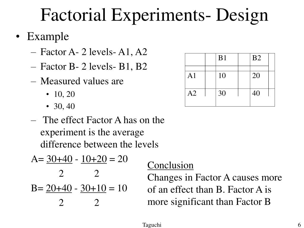
The Main Total Effect can be related to input variables by moving along the row and looking at the first column. If the row in the first column is a2b1c1 then the main total effect is A. To get a mean factorial effect, the totals needs to be divided by 2 times the number of replicates, where a replicate is a repeated experiment. This can be seen by noting that the pattern of entries in each A column is the same as the pattern of the first component of "cell". (If necessary, sorting the table on A will show this.) Thus these two vectors belong to the main effect of A. Similarly, the two contrast vectors for B depend only on the level of factor B, namely the second component of "cell", so they belong to the main effect of B.
Factorial experiment
The advantage of this is that multiple-response measures are generally more reliable than single-response measures. However, it is important to make sure the individual dependent variables are correlated with each other by computing an internal consistency measure such as Cronbach’s \(\alpha\). If they are not correlated with each other, then it does not make sense to combine them into a measure of a single construct. If they have poor internal consistency, then they should be treated as separate dependent variables.
To illustrate, a 3 x 3 design has two independent variables, each with three levels, while a 2 x 2 x 2 design has three independent variables, each with two levels. Time of day (day vs. night) is represented by different locations on the x-axis, and cell phone use (no vs. yes) is represented by different-colored bars. It would also be possible to represent cell phone use on the x-axis and time of day as different-colored bars. The choice comes down to which way seems to communicate the results most clearly.
Statistical modeling and optimization of heterogeneous Fenton-like removal of organic pollutant using fibrous catalysts ... - Nature.com
Statistical modeling and optimization of heterogeneous Fenton-like removal of organic pollutant using fibrous catalysts ....
Posted: Wed, 30 Sep 2020 07:00:00 GMT [source]
The random assignment of participants to the treatment arms means that the two groups of assigned participants should differ systematically only with regard to exposure to those features that are intentionally withheld from the controls. In smoking cessation research a common RCT design is one in which participants are randomly assigned to either an active pharmacotherapy or to placebo, with both groups also receiving the same counseling intervention. The interaction effects situation is the last outcome that can be detected using factorial design. From the example above, suppose you find that 20 year olds will suffer from seizures 10% of the time when given a 5 mg CureAll pill, while 20 year olds will suffer 25% of the time when given a 10 mg CureAll pill.
Further, this problem is reduced if factorial designs are used as screening experiments, whose purpose is not to identify the single best combination of ICs (Collins et al., 2009). Rather such experiments are used to identify the ICs that are amongst the best. Therefore, finding that several combinations of ICs yield promising effects is compatible with the goal of a screening experiment, which is to distill the number of ICS to those holding relatively great promise. In keeping with this, the data in Figure 1 suggest that we can winnow potentially promising combinations from 16, to 3. Which one of those three might be deemed most promising might be addressed via other criteria (effects on abstinence, costs, and so on) and in a follow-up RCT.
For instance, not only do such designs permit the screening of multiple intervention components in a single experiment, but compared with RCT designs, factorial experiments permit more precise estimates of mediational effects. This paper highlights decisions and challenges related to the use of factorial designs, with the expectation that their careful consideration will improve the design, implementation, and interpretation of factorial experiments. In addition, the complexity of delivering multiple combinations of components can be reduced by using a fractional factorial design (Collins et al., 2009), which reduces the number of different component combinations per the number of factors used. While more research on IC interactions is surely needed, our research has consistently found such interactions (Cook et al., 2016; Fraser et al., 2014; Piper et al., 2016; Schlam et al., 2016). Thus, it might be difficult in many cases to assume conditions that would justify the use of a fractional factorial design. When taking a general linear model approach to the analysis of data from RCTs and factorial experiments, analysts must decide how to code categorical independent variables.
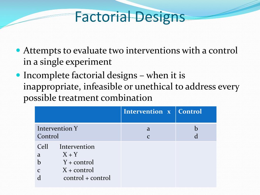
This design can be represented in a factorial design table and the results in a bar graph of the sort we have already seen. The researcher would consider the main effect of sex, the main effect of self-esteem, and the interaction between these two independent variables. Thus far we have seen that factorial experiments can include manipulated independent variables or a combination of manipulated and non-manipulated independent variables. But factorial designs can also include only non-manipulated independent variables, in which case they are no longer experiments but are instead non-experimental in nature. This can be conceptualized as a 2 × 2 factorial design with mood (positive vs. negative) and self-esteem (high vs. low) as non-manipulated between-subjects factors.


No comments:
Post a Comment